For full source-code check my repository.
This post is based on the Pixel Recurrent Neural Networks paper.
This post is not about explaining PixelCNN and I won’t dive into the theory too much, the paper I linked above does a good job of that, this post is rather an extension of the paper, from theory to implementation.
After reading this post, you will know how to implement PixelCNN in Keras, how to train it so it generates naturally looking images, and how to tackle the challenges of a project like this.
Getting Started
Keras has two ways of defining models, the Sequential, which is the easiest but limiting way, and the Functional, which is more complex but flexible way.
We will use the Functional API because we need that additional flexibility, for example - the Sequential model limits the amount of outputs of the model to 1, but to model RGB channels, we will need 3 output units, one for each channel. As the model gets more complex (e.g Gated PixelCNN) it will become clearer why Functional API is a no-brainer for projects like this.
Our input shape(excluding batch) should be: (height, width, channels).
More specifically, MNIST (grayscale) input shape looks like this (28, 28, 1) and CIFAR (32, 32, 3).
Let’s start simple, we’ll do a PixelCNN for grayscale MNIST first.
shape = (28, 28, 1)

input_img = Input(shape)
Architecture
Since the paper focuses on PixelRNN, it fails to provide a clear explanation on how the architecture of PixelCNN should look like, however, it does a good job of describing the big picture, but it is not enough for actually implementing PixelCNN.
Here’s the architecture I came up with for grayscale MNIST (with only 1 residual block for simplicity):
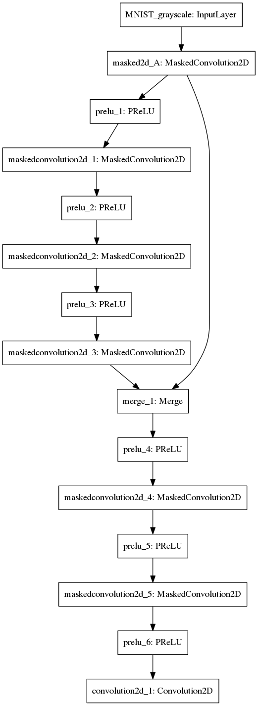
Note that PixelCNN has to preserve the spatial dimension of the input, which is not shown in the graph above.
Masked Convolutions
We already defined our input, and as you can see in the architecture graph, the next layer is a masked convolution, which is the next thing we are going to implement.
How to implement grayscale masks?
Here’s a picture for reference:
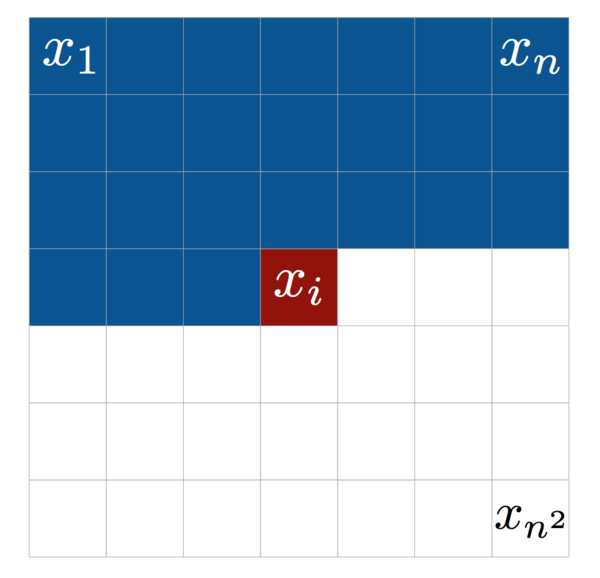
The difference between type A and B masks in grayscale images is that type A also masks the center pixel.
Keep in mind that masks for grayscale images are simpler than RGB masks, but we’ll get to RGB masks too.
Here’s how we are going to implement masks:
- Create a numpy array of ones in the shape of our convolution weights:
(height, width, input_channels, output_channels) - Zero out all weights to the right and below of the center weights (to block future insight of pixels from flowing, as stated in the paper).
- If the mask type is
A, we’ll zero out the center weights too (to block insight of the current pixel as well). - Multiply the mask with the weights before calculating convolutions.
Let’s use the steps above to go ahead and implement a new Keras layer for masked convolutions:
import math

import numpy as np

from keras import backend as K
from keras.layers import Convolution2D

class MaskedConvolution2D(Convolution2D):
    def __init__(self, *args, mask='B' , n_channels=3, mono=False, **kwargs):
        super().__init__(*args, **kwargs)
        self.mask_type = mask

        self.mask = None

    def build(self, input_shape):
        super().build(input_shape)

        # Create a numpy array of ones in the shape of our convolution weights.
        self.mask = np.ones(self.W_shape)

        # We assert the height and width of our convolution to be equal as they should.
        assert mask.shape[0] == mask.shape[1]

        # Since the height and width are equal, we can use either to represent the size of our convolution.
        filter_size = self.mask.shape[0]
        filter_center = filter_size / 2

        # Zero out all weights below the center.
        self.mask[math.ceil(filter_center):] = 0

        # Zero out all weights to the right of the center.
        self.mask[math.floor(filter_center):, math.ceil(filter_center):] = 0

        # If the mask type is 'A', zero out the center weigths too.
        if self.mask_type == 'A':
            self.mask[math.floor(filter_center), math.floor(filter_center)] = 0

        # Convert the numpy mask into a tensor mask.
        self.mask = K.variable(self.mask)

    def call(self, x, mask=None):
        ''' I just copied the Keras Convolution2D call function so don't worry about all this code.
            The only important piece is: self.W * self.mask.
            Which multiplies the mask with the weights before calculating convolutions. '''
        output = K.conv2d(x, self.W * self.mask, strides=self.subsample,
                          border_mode=self.border_mode,
                          dim_ordering=self.dim_ordering,
                          filter_shape=self.W_shape)
        if self.bias:
            if self.dim_ordering == 'th':
                output += K.reshape(self.b, (1, self.nb_filter, 1, 1))
            elif self.dim_ordering == 'tf':
                output += K.reshape(self.b, (1, 1, 1, self.nb_filter))
            else:
                raise ValueError('Invalid dim_ordering:', self.dim_ordering)
        output = self.activation(output)
        return output

    def get_config(self):
        # Add the mask type property to the config.
        return dict(list(super().get_config().items()) + list({'mask': self.mask_type}.items()))
First Masked Convolution Layer
Now that we have masked convolutions implemented, let’s add the first masked convolution to our model(which is practically just an input layer at the moment).
According to the paper, the layer after the input is a masked convolution of type A, with a filter size of (7,7) and it has to preserve the spatial dimensions of the input, we’ll use border_mode='same' for that.
Note that this layer is the only masked convolution of type A the model will have.
shape = (28, 28, 1)
filters = 128

input_img = Input(shape)

model = MaskedConvolution2D(filters, 7, 7, mask='A', border_mode='same')(input_img)
Now we should have a simple graph like this: input -> masked_convolution.
Residual blocks
After the first masked convolution the model has a series of residual blocks (The architecture picture above has only 1 residual block).
To implement a residual block:
- Take input of shape
(height, width, filters). - Halve the filters with a
(1,1)convolution. - Apply a
(3,3)masked convolution of typeB. - Scale the filters back to original with
(1,1)convolution. - Merge the original input with the convolutions.
The reason for cutting the filters by half and then scaling back to original is because it is a good way to get a computational boost while not significally reducing model performance.
Let’s implement a residual block in Keras:
class ResidualBlock(object):
    def __init__(self, filters):
        self.filters = filters

    def __call__(self, model):
        # filters -> filters/2
        block = PReLU()(model)
        block = Convolution2D(self.filters//2, 1, 1)(block)

        # filters/2 3x3 -> filters/2
        block = PReLU()(block)
        block = MaskedConvolution2D(self.filters//2, 3, 3, border_mode='same')(block)

        # filters/2 -> filters
        block = PReLU()(block)
        block = Convolution2D(self.filters, 1, 1)(block)

        # Merge the original input with the convolutions.
        return Merge(mode='sum')([model, block])
We will want to stack those residual blocks in our model, so let’s create a simple layer for that:
class ResidualBlockList(object):
    def __init__(self, filters, depth):
        self.filters = filters
        self.depth = depth

    def __call__(self, model):
        for _ in range(self.depth):
            model = ResidualBlock(self.filters)(model)

        return model
Stacking Residual Blocks
Now let’s stack those residual blocks on our model.
We also need to add an activation after the stack, because the residual block ends with a convolution, not an activation.
shape = (28, 28, 1)
filters = 128
depth = 6

input_img = Input(shape)

model = MaskedConvolution2D(filters, 7, 7, mask='A', border_mode='same')(input_img)

model = ResidualBlockList(filters, depth)
model = PReLU()(model)
Wrapping Up for Output
As shown in the architecture picture above, the model has additional 2 masked convolutions before output.
According to the paper, those 2 masked convolutions are of size (1,1) and of type B.
Let’s add those to our model:
shape = (28, 28, 1)
filters = 128
depth = 6

input_img = Input(shape)

model = MaskedConvolution2D(filters, 7, 7, mask='A', border_mode='same')(input_img)

model = ResidualBlockList(filters, depth)
model = PReLU()(model)

for _ in range(2):
    model = MaskedConvolution2D(filters, 1, 1, border_mode='valid')(model)
    model = PReLU()(model)
Output
Since we have just one channel, we can convolve the pixels with a convolution of size (1,1) with a single filter and then sigmoid its output.
The output of the sigmoid should be a 2D array with an exact shape as the input ((28, 28, 1) for MNIST), with each point in the 2D array representing a (grayscale) color value.
It shoud look like this:
shape = (28, 28, 1)
filters = 128
depth = 6

input_img = Input(shape)

model = MaskedConvolution2D(filters, 7, 7, mask='A', border_mode='same')(input_img)

model = ResidualBlockList(filters, depth)
model = PReLU()(model)

for _ in range(2):
    model = MaskedConvolution2D(filters, 1, 1, border_mode='valid')(model)
    model = PReLU()(model)

outs = Convolution2D(1, 1, 1, border_mode='valid')(model)
outs = Activation('sigmoid')(outs)
Compiling The Model
I chose Nadam quite arbitrarily, you can go with any optimizer you like.
Since we use sigmoid in our output activations our loss should be binary_crossentropy.
Let’s compile the model:
model = Model(input_img, outs)
model.compile(optimizer=Nadam(), loss='binary_crossentropy')
Training the model
Loading MNIST data with Keras
Let’s load MNIST data, change data type to float and normalize it.
We ignore the labels of MNIST because they are not useful for our case, our model is not a classifier.
Note that I concatenate the training and test data, I do that to have more data to help with training, however, if you need validation data, feel free to not concatenate them.
(train, _), (test, _) = mnist.load_data()
data = np.concatenate((train, test), axis=0)
data = data.astype('float32')
data /= 255
Fit The Model to MNIST
Set the arguments needed for training, I also added a TensorBoard and a ModelCheckpoint callbacks to the training routine.
We pass the data both as our input and target output.
This setup is similar to an autoencoder’s one, but PixelCNN is not an autoencoder, it doesn’t learn an effcient encoding of the data but rather learns the distribution of the values in the data.
Here’s how the fit routine should look like:
batch_size = 32
epochs = 200
callbacks = [TensorBoard(), ModelCheckpoint('model.h5')]

model.fit(data, data,
      batch_size=batch_size, nb_epoch=epochs,
      callbacks=callbacks)
Generating MNIST
To generate images PixelCNN needs to predict each pixel separately, more concretly, you will need to feed it an 2D array of zeros, let it predict the first pixel, refeed the array, predict second pixel, and so on…
PixelCNN outputs an array of pixel value probabilities for each pixel, to generate different images we should not use argmax when picking a pixel value, but rather pick a pixel value using the probabilities themselves.
Keep in mind, generating images does not benefit from the convolution’s concurrent nature and everything has to be done sequentially pixel by pixel.
# Using a batch size allows us to predict a few pixels concurrently.
batch = 8

# Create an empty array of pixels.
pixels = np.zeros(shape=(batch,) + (model.input_shape)[1:])
batch, rows, cols, channels = pixels.shape

# Iterate the pixels because generation has to be done sequentially pixel by pixel.
for row in range(rows):
    for col in range(cols):
        for channel in range(channels):
            # Feed the whole array and retrieving the pixel value probabilities for the next pixel.
            ps = model.predict_on_batch(pixels)[channel][:, row*cols+col]

            # Use the probabilities to pick a pixel value.
            # Lastly, we normalize the value.
            pixels[:, row, col, channel] = np.array([np.random.choice(256, p=p) for p in ps]) / 255

# Iterate the generated images and plot them with matplotlib.
for pic in pixels:
    plt.imshow(pic, interpolation='nearest')
    plt.show(block=True)
What’s Next
That’s all about Grayscale PixelCNN.
In another post I’ll explain how to implement a multi-channel(RGB) PixelCNN.
To do so, the following changes would be made:
- Multi-channel masks.
- Multi-channel output.
- Masks throughout the residual blocks.
Until next time, happy training.